Dense Retrieval

November 18, 2025 by Laurynas Jasiukėnas and Dainius Jocas

TL;DR: integrating embedding-based retrieval into the e-commerce search application is a significant undertaking.

Introduction

The low-recall aspect of the keyword-based search is challenging when dealing with the content which is both very visual and multilingual. Returning “no results” even when there are relevant items is a missed business opportunity. To address the challenge, the initial experimentation with the dense embeddings-based retrieval can be tracked back to internal hackathons as early as 2022.

To prove the business value and to maximise learning, we implemented filling of low-recall search sessions with some dense retrieval matches. A little increase in recall turned into improved search metrics which gave more confidence in the technique.

Attempts to include dense retrieval matches in all search sessions started in the spring of 2024. When a technical approach and business value was proven in one market with one dominant language, it was time to work on scaling the solution.

Some 50 AB tests later, the dense retrieval is fully enabled. It required numerous model improvements and a bunch of engineering wizardry which are covered in the remainder of this post.

ML Model

At its core, our system is a Two-Tower Model:

The Query Tower: Takes a user’s search query (e.g. “red summer dress”) and encodes it into a 256-dimension vector (a.k.a. “query embedding”).
The Item Tower: Takes an item from our catalog and encodes all its features into a vector (a.k.a. “item embedding”) of the same 256 dimensions.

The Query Tower

The frozen pre-trained multilingual CLIP model is our base for further fine-tuning. We train a “projection head” with GELU activations and LayerNorm. That not only complements CLIP’s general-purpose knowledge with our search domain specifics, but also makes training fast and efficient.

The Item Tower

An item’s representation is a fusion of signals, including its image and metadata (brand, color, category, price, etc.):

Categorical Features: Embeddings from data like brand ids, category ids, etc., each projected to a 256-dimensional space
Visual Features: Pre-calculated CLIP embeddings from our primary product images (512 dimensions input projected to 256 dimensions).

These vectors are concatenated and passed through a final fusion layer. This allows the model to learn the complex interactions between all features (e.g., how a specific brand relates to a specific image style).

Including the textual item information into the model turned out to be challenging but remains a promising direction for future improvements, perhaps a much larger training dataset or different incorporation techniques are worth a try.

The Training Recipe

The two towers are trained together using contrastive learning. The model learns to pull positive (relevant) query-item pairs together while pushing negative (irrelevant) pairs apart. For every (query, positive_item) pair, we force the model to distinguish it from 7,000–10,000 random negative items.

To get this training to converge, we use a full recipe of such practices:

A learnable temperature parameter that self-tunes the “difficulty” of the loss.
Mixed-precision (FP16) training for a speed-up.
The AdamW optimizer with separate weight decay.
A Cosine Annealing learning rate scheduler for stable convergence.

With the same training recipes we saw model training improvements by scaling dataset by 10x to more than 100 million positive pairs.

For deployment, converting the item model to ONNX introduced complexities in handling categorical feature preprocessing. Our solution is to integrate the preprocessing logic directly into the ONNX graph by using a masking technique to filter and manage out-of-vocabulary (OOV) inputs.

Removing irrelevant nearest neighbors requires picking an arbitrary similarity value. Doing this not only requires manually-tuning combined further adjustments with AB testing, but also mandates adjustment after every model retraining. Furthermore, it could be adjusted per query based on some estimated recall value during query time.

System architecture

The entire implementation is within a Vespa application package.

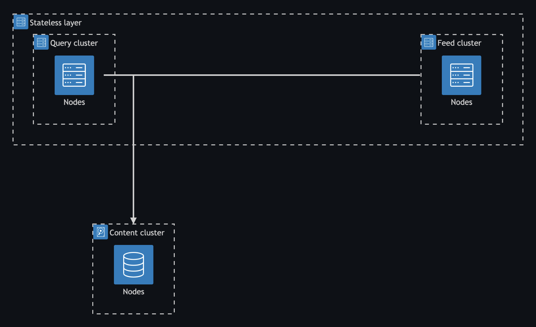
In the high-level architecture diagram above we see that within the Vespa stateless layer query and feeding containers are physically separated. The separation allows adding resources individually and on demand. Query cluster nodes run the query model configured as a standard Vespa embedder. The feed cluster nodes contain the item tower that is invoked in a custom Vespa document processor that invokes a model evaluator whose result is added to the document update operation. Both query and feed nodes communicate with the same content cluster. The content cluster nodes contain HNSW index on the portion of the dataset. All models files and configuration is managed within a single Vespa application package.

It is also worth mentioning that to initially calculate image embeddings of only the primary photo for all the items took about 1 month. The image embeddings weigh around ~ 1 TB of memory (10^9 items * 512 dimensions * 2 bytes per dimension). The item embeddings weight half as much.

Performance

Combining the fast HNSW search with filtering is a major performance challenge. This combination requires extensive optimization, even in a high-performance system like Vespa, to stay within a tight latency budget. Below we list such optimizations roughly sorted by complexity.

Add nodes to content groups

The worst-case scenario for ANN search has high tail latencies because a lot of vector comparisons are needed. One simple approach to lower the latency is to make HNSW smaller by splitting the data into more content nodes and executing more searches in parallel. Currently, we have 30 nodes per content group.

Split the index

Vinted has some markets connected, e.g. members in Spain can see French items. Markets that are transitively connected form a logical bloc. We leveraged that to create smaller HNSW indices per bloc. This was achieved by creating 3 separate Vespa indices that are deployed to the same content cluster.

This trick not only made HNSW searches more manageable, but as a side effect, it also sped up all search requests. However, the indexing and querying now need to be routed to the correct indices.

Tune thresholds

Vespa dynamically decides which nearest neighbor searches strategy to apply based on the estimated hit ratio. Thresholds can be tuned to balance latency vs. resource utilization. During the benchmarking we’ve discovered that the sweet spot was to set ranking.matching.approximateThreshold to a values that translates to ~1M documents per index per content node with 8 threads per search request.

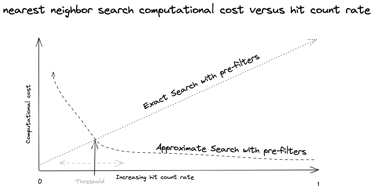
Note that there is no perfect threshold.

Retry strategy

Search requests have a tight latency budget of 500 ms. Even with the tuned thresholds, we’d still get some timeouts due to how the approximate nearest neighbor search is executed. The worst part is that such failures end in 0 results sessions. Knowing that the exact nearest neighbor search doesn’t have such a failure mode we implemented a retry strategy:

Divide latency budget into 2 parts: e.g. 350 ms and 150 ms
First, prefer executing the approximate nearest neighbor search with a timeout of 350 ms
If the first request fails, then force the exact nearest neighbor search by ranking.matching.approximateThreshold=1 with a timeout of 150 ms.

The sequence diagram below explains the flow.

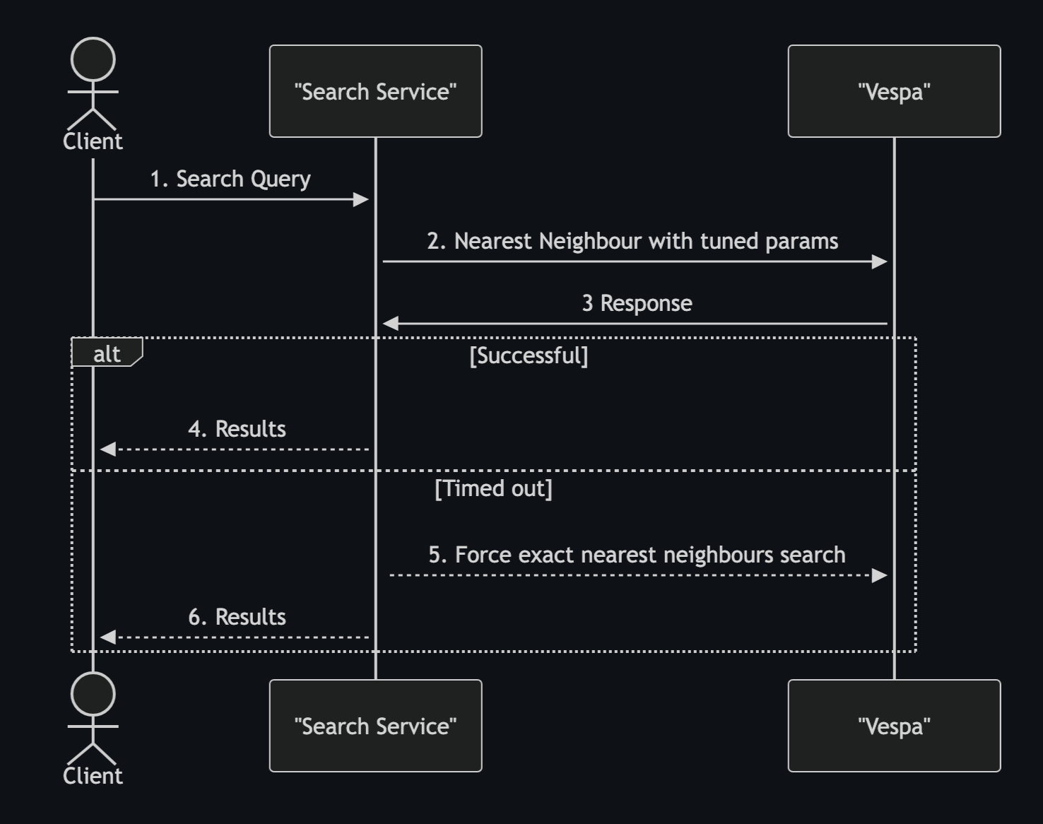
Typically, a Vespa timeout means that the summary fetching was skipped. Such responses are mostly unusable as the document data is not in the response. To “recover” such requests, we leveraged the match-features to return a document ID as a tensor. The strategy eliminated most of the timeouts.

Consistency

The key requirement was to integrate the dense retrieval into the existing setup. This means:

Support a hard limit on the number of dense retrieval matches added to the Top-K results as simply flooding results with approximate matches is a bad user experience.
Adding a filter should not increase the number of search results.
Avoid surprise when changing the sorting of search results.

It might be hard to believe, but all of the above happened for real user queries.

Example

A query zx750 with a brand filter has ~300 lexical matches and with the tuned distance threshold the nearest neighbor search matches another ~7000 items. The problem with those 7000 items is that they are mostly random things, and the lexical matches are spread across those ~7300 hits. The poor matches are due to BERT-based tokenizer producing tokens [CLS]z##x##75##0[SEP] that tend to give high similarity with random items. If the brand filter is removed, we get the expected ~450 (~300 lexical and ~150 nearest neighbor) matches.

Nearest neighbor target hits

It turns out that the dynamic switching between exact and approximate the nearest neighbor search strategies introduces these failure modes. It boils down to how the targetHits param is handled in each strategy. Each nearestNeighbor query clause has the targetHits param. However, it is only a target, not a limit! Meaning that Vespa is free to add nearest neighbor matches. And it happens when the execution strategy is the exact nearest neighbor. For example, when a filter is added to the search request, surprisingly, there can be more matches than without a filter. Also, targetHits is per content node. So, the total limit is targetHits * number_of_content_nodes. Not ideal. Note that the approximate nearest neighbor execution strategy returns exactly targetHits Per content node.

This behaviour originates in the matching phase. So, later in the ranking we can already implement a workaround.

Approach

Having consistency requirements and the technical limitation in mind, there were only a few paths to go:

Ignore the problem
Two requests to Vespa and combine the results in the application layer
Push the complexity down to Vespa

Taking the blue pill and ignoring the problem (1) was not really an option as it would mean either killing a promising project or leaving the expensive feature as a filler for low results queries. (2) Two requests felt unattractive as it would introduce plenty of complexity (e.g. faceting) to make the codebase toxic to the extent that nobody would dare to touch it.

We decided to proceed with taking the red pill and creatively pushing the complexity down to Vespa (3). We believe that reading Vespa documentation and following a ranking profile is easier than reading a hacky implementation code.

Reciprocal rank fusion

A.k.a. RRF is a Vespa ranking feature available in the global-phase. It is defined as rrf_score = 1.0 / (k + rank). The score depends on an arbitrary parameter k and the rank (position) within a virtual list of search results ranked by some ranking feature, e.g. nearest neighbor similarity.

If you squint, when k=0 then rrf_score looks like a position. We can find a number that represents N-th position rrf_score@N=1/N, e.g. rrf_score@160=1/160=0.00625.

Identifying the nearest neighbor matches

All documents matched by the nearestNeighbor query clause has a non 0 itemRawScore rank feature. However, to answer if the document is matched only by the nearestNeighbor the we need to know if the document was not matched by other query clauses.

The YQL conceptually looks like this:

SELECT *
FROM documents
WHERE filters AND (lexical_match OR interpretations OR nearestNeighbor) 

If a document is a lexical match then textSimilarity(text_field).queryCoverage > 0 must be true.

By interpretations we mean a query rewrites into filters on metadata, e.g. a query `red dress` becomes a filter color_id=10 AND category_id=1010. The complication is that there might be multiple interpretations, and we need to know if the document is a full match of at least one interpretation. There is no easy way to calculate such condition. A workaround is to introduce a boolean attribute field where the value is always false.

field bool_const type bool {
  indexing: attribute
  attribute: fast-search
  rank: filter
}

Then rewrite each interpretation AND’ing with the always TRUE bool_const=FALSE condition, e.g.

color_id=10 AND category_id=1010 AND bool_const=FALSE

Now, if the rank feature attributeMatch(bool_const) > 0 then the document is fully matched by at least one interpretation. To distinguish between interpretations a field per interpretation would be needed.

Finally, we can identify if the document is only a nearest neighbor match:

function match_on_nearest_neighbor_only() {
  expression {
    if(itemRawScore(dense_retrieval) > 0 
          && textSimilarity(text_field).queryCoverage == 0
          && attributeMatch(bool_const) == 0,
      1,
      0
    )
  }
}

Using the global ranking phase as a filter

Matches from all content nodes are available in the container node in the global ranking phase. It supports a rank-score-drop-limit parameter that can be used to remove matched documents whose score is lower than some constant numeric value. This feature was contributed to Vespa.

The trick to filter out documents is to change the score of some matches to a value lower than the rank-score-drop-limit.

A nice thing is that this parameter can be passed as an HTTP request parameter to have a control per request or for AB testing.

Putting all together

Here is the implementation that limits the nearest neighbor matches count using the tricks described above:

global-phase {
  expression {
    if(reciprocal_rank(itemRawScore(dense_retrieval), 0) >= 1.0 / query(nn_hits_limit)
          || match_on_nearest_neighbor_only == 0,
    relevanceScore,
    -100000.0)
  }
  rerank-count: 20000
  rank-score-drop-limit: -100000.0
}

It works like this: when the document is either a nearest neighbor match up to query(nn_hits_limit) position or it is not only a nearest neighbor match then the document gets the same score as calculated in the previous ranking phases (i.e., no change). Otherwise, the score is set to -100000.0 (way outside the range of the normal scores). We take 20,000 documents (meaning “all”) to rerank. After reranking the documents with score <-100000 are filtered out.

Sorted queries

Yet another complication is that every result ordering has to deal with the same issue of limiting the number of nearest neighbor matches. The required sorting has to be implemented with ranking profiles because global-phase prevents using the order by clause. Here is an example rank profile for the “newest first” sorting:

rank-profile dense_retrieval_newest inherits dense_retrieval_global_phase {
    match-phase {
        attribute: first_visible_at
        order: descending
    }
    first-phase {
        expression: attribute(first_visible_at)
    }
}

Another way to see this complication is that it creates an opportunity for secondary sorting to use some clever scoring that might include personalization or something. While secondary sorting with order by are limited to an indexed attribute value.

Custom JVM

Using the global-phase reranking as a filter added quite a bit of work to the query container nodes which increased latencies. To amortise for that, we’ve experimented with a newer JVM as Vespa ships with a relatively old OpenJDK 17.

In the past, we’ve had great results with GraalVM when running Elasticsearch. Why not try it with Vespa? And it turns out that it works pretty well! The tail latencies dropped by double-digit percentages. Later we’ve also configured ZGC so that JVM garbage collection pauses would cause fewer timeouts.

Using the combination of GraalVM and ZGC not only helped with this project but also proved to help with other ultra low-latency use cases.

Peak of Complexity

Even though the current implementation gets the job done, we are not happy. The logic is not particularly complicated, but it has many components, and therefore it is easy to get lost. We’ve added plenty of integration tests that prevent introducing bugs when changing something remotely related.

The worst part of it is that additional requirements can be implemented only by adding even more complexity. To get rid of this complexity, either the consistency requirements need to change, or performance of ANN should be significantly improved, or the model is improved so that all items that pass distance thresholds are relevant.

This reminds of the Peak of Complexity model introduced by the Java architect Brian Goetz. We’ve just passed the complexity peak, and we’re in the virtuous collapse phase where simplification leads to even more simplification. When looking into parts of the solution, it is not uncommon to hear questions like what took you so long?

Summary

The dense retrieval is a significant improvement to the item search. The benefits were proved in lots of AB tests. However, as it is typical for search, good work leads to even more work: the model can get better, the integration into the ranking can be improved, nuance can be introduced when and to what extent the dense retrieval is applied, resource utilization can be optimized, etc.

Even though a lot of work is ahead of us, we are proud of what has been achieved. The overall architecture is relatively simple and contained, which allows for the team autonomy. Due to multiple performance optimizations, we’ve reached a <0.02% error rate. The techniques mastered for this feature have laid the foundations for other advancements such as image search or advanced personalization.

We hope that this long blog post was interesting and sheds some light on what it takes to work out a significant search feature at the billion-scale e-commerce dataset.

Vinted Engineering

These are the voyages of code tailors that help create Vinted