Sharding out Elasticsearch
Finding the right settings of indices is a relentless process of monitoring and experimenting. I want to share key methods of detecting scalability problems of Elasticsearch using metrics and automation.
We use Elasticsearch for ranking product listings and full-text search for products, forum posts and user messages. Most complex queries include scoring functions, various filters and weight boosters. Before Elasticsearch we have used Sphinx, but due to demand for more dynamic querying logic we migrated to ES 1.7.x, now 5.4.0.
The production cluster consists of 21 nodes: 3 masters, 3 coordinating (client) and 15 data nodes (all of them are ingest nodes as well). Hardware configuration is the same for all data nodes. Only data nodes run on physical servers. The cluster serves 10 countries, has 397 million documents, occupies about 0.93TB of size on disk.
On indices level, we have 46 indices, 635 shards of which 212 are primary.
Noticing ineffective resource usage
I will approach Elasticsearch from the most basic hardware resources CPU & RAM. Elasticsearch has a limit of total memory it can use it is ~32GB (heap-sizing). Spare memory is used for OS cache and Lucene in-memory data structures. If a single node has indices that add up to the size bigger than 32GB, then GC collections occur more often. Or young generation is garbage collected before it is moved to old. In our case, the latter occurred - it is visible from the following graphs.
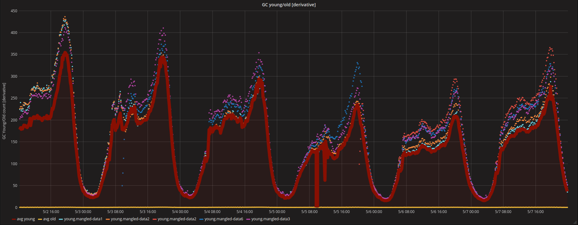
The red thick line is an average of the young generation, points above are top 5 average nodes. In our case, this means that those nodes have more shards allocated to them. The following sections elaborates on this more.
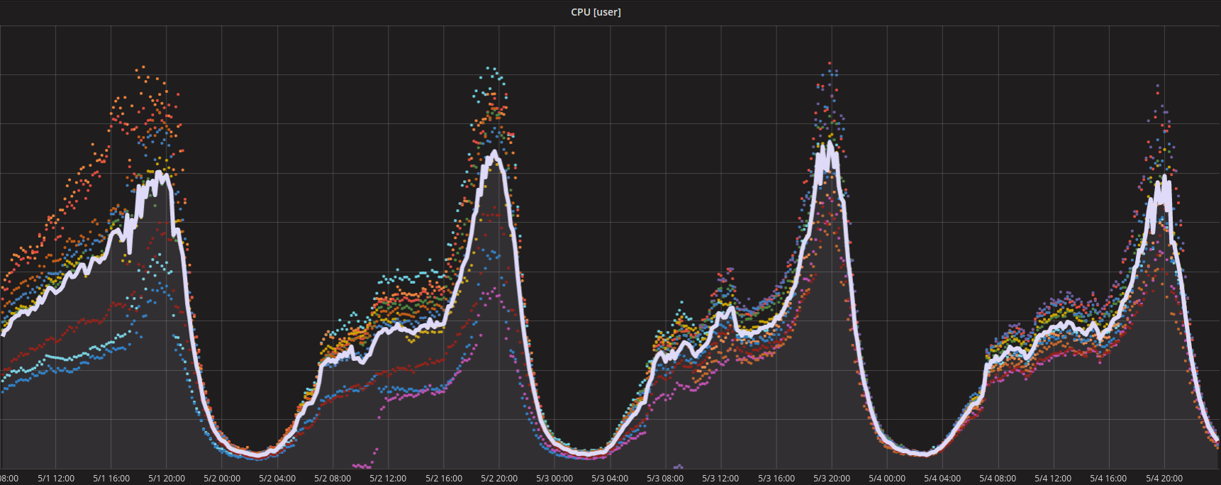
The same pattern can be seen from CPU usage graphs.
Checking shards distribution
Elasticsearch provides /_cat/indices API to view indice settings.
green open large-index_20170523104530 Yq5viGdtRTWXsBeTIUT8HA 5 2 20009347 xxxxxxxx  67.6gb 22.5gb
green open large-index_20160719210848 Y3EWgkNiRKOPodeWEuDWyg 3 9 20004745 xxxxxxxx 274.8gb 27.6gb
From the above example, it can be seen that there are two versions of the same indice (note indices without timestamp - large-index_ indicates that it is the same index), the core difference is in shards and replication count settings.
For shorter notation large-index_20170523104530 indice will be
2017and large-index_201607192108482016respectively.
2017 indice has 5 shards and replication count 2 where 2016 has 3 shards and 9 as a replication count.
To find out how shards are distributed we can consult Elasticsearch provided /_cat/shards API.
2016
large-index_20160719210848 2 r STARTED 6665383 7.9gb dc1-data2
large-index_20160719210848 2 r STARTED 6665383 8.3gb dc2-data4
large-index_20160719210848 2 r STARTED 6665383 7.7gb dc3-data1
large-index_20160719210848 2 r STARTED 6665383 8gb dc2-data3
large-index_20160719210848 2 r STARTED 6665383 7.8gb dc2-data1
large-index_20160719210848 2 r STARTED 6665383 7.8gb dc1-data1
large-index_20160719210848 2 r STARTED 6665383 7.8gb dc3-data5
large-index_20160719210848 2 r STARTED 6665383 8.4gb dc3-data2
large-index_20160719210848 2 p STARTED 6665383 7.9gb dc2-data6
large-index_20160719210848 2 r STARTED 6665383 7.9gb dc2-data5
large-index_20160719210848 1 r STARTED 6671132 10.3gb dc1-data2
large-index_20160719210848 1 r STARTED 6671132 10.6gb dc2-data3
large-index_20160719210848 1 r STARTED 6671132 10.4gb dc3-data3
large-index_20160719210848 1 r STARTED 6671132 10.6gb dc3-data4
large-index_20160719210848 1 r STARTED 6671132 9.8gb dc2-data6
large-index_20160719210848 1 r STARTED 6671132 10.1gb dc2-data2
large-index_20160719210848 1 r STARTED 6671132 10.2gb dc2-data5
large-index_20160719210848 1 r STARTED 6671132 10.1gb dc2-data8
large-index_20160719210848 1 r STARTED 6671132 10.3gb dc2-data7
large-index_20160719210848 1 p STARTED 6671132 10.5gb dc3-data6
large-index_20160719210848 0 r STARTED 6668230 8.8gb dc3-data1
large-index_20160719210848 0 r STARTED 6668230 8.9gb dc2-data1
large-index_20160719210848 0 r STARTED 6668230 9gb dc1-data1
large-index_20160719210848 0 r STARTED 6668230 8.9gb dc3-data5
large-index_20160719210848 0 r STARTED 6668230 9.4gb dc3-data2
large-index_20160719210848 0 r STARTED 6668230 9gb dc3-data4
large-index_20160719210848 0 r STARTED 6668230 9.4gb dc2-data2
large-index_20160719210848 0 p STARTED 6668230 9.1gb dc2-data8
large-index_20160719210848 0 r STARTED 6668229 9.4gb dc2-data7
large-index_20160719210848 0 r STARTED 6668229 9.3gb dc3-data6
From shards distribution on data nodes we see that they are duplicated.
2017
large-index_20170523104530 3 r STARTED 4002941 4.5gb dc2-data4
large-index_20170523104530 3 r STARTED 4002941 4.5gb dc3-data2
large-index_20170523104530 3 p STARTED 4002941 4.5gb dc3-data4
large-index_20170523104530 2 p STARTED 4003777 4.5gb dc3-data3
large-index_20170523104530 2 r STARTED 4003777 4.5gb dc2-data2
large-index_20170523104530 2 r STARTED 4003777 4.5gb dc2-data7
large-index_20170523104530 4 r STARTED 4000280 4.5gb dc3-data1
large-index_20170523104530 4 r STARTED 4000280 4.5gb dc2-data6
large-index_20170523104530 4 p STARTED 4000280 4.5gb dc2-data5
large-index_20170523104530 1 r STARTED 4000258 4.5gb dc1-data2
large-index_20170523104530 1 p STARTED 4000258 4.5gb dc1-data1
large-index_20170523104530 1 r STARTED 4000258 4.5gb dc3-data5
large-index_20170523104530 0 p STARTED 4002092 4.5gb dc2-data3
large-index_20170523104530 0 r STARTED 4002092 4.5gb dc2-data1
large-index_20170523104530 0 r STARTED 4002092 4.5gb dc2-data8
Shards have 30% fewer documents and half the size comparing with 2016.
Let’s compare shards duplications of 2016 and 2017 indices.
2016
$ grep large-index_20160719210848 shards | awk '{print $8}' | sort | uniq -c
      2 dc1-data1
      2 dc1-data2
      2 dc2-data1
      2 dc2-data2
      2 dc2-data3
      1 dc2-data4
      2 dc2-data5
      2 dc2-data6
      2 dc2-data7
      2 dc2-data8
      2 dc3-data1
      2 dc3-data2
      1 dc3-data3
      2 dc3-data4
      2 dc3-data5
      2 dc3-data6
2017
$ grep -v large-index_20160719210848 shards | awk '{print $8}' | sort | uniq -c
      1 dc1-data1
      1 dc1-data2
      1 dc2-data1
      1 dc2-data2
      1 dc2-data3
      1 dc2-data4
      1 dc2-data5
      1 dc2-data6
      1 dc2-data7
      1 dc2-data8
      1 dc3-data1
      1 dc3-data2
      1 dc3-data3
      1 dc3-data4
      1 dc3-data5
It is evident that 2017 is evenly distributed.
Knowing how shards will be allocated to nodes
I have come up with a formula of allocating 1 shard per node. One shard per node allows more efficient request serving and scaling.
def nodes(shards, replicas)
  shards * replicas + shards
end
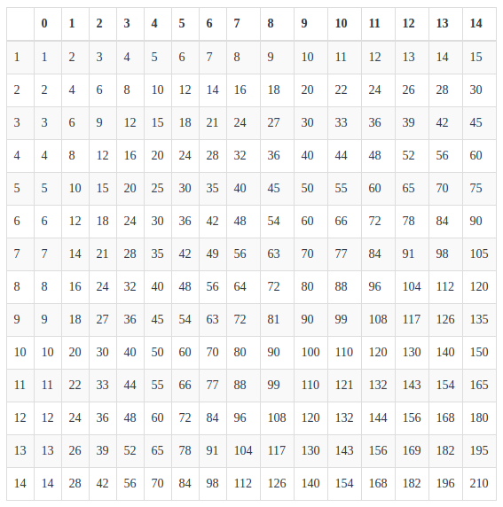
The table above shows node count needed to have 1 shard/node for indice.
X axis - replica count
Y axis - shard count
So for 2016 indice with 3 shards and 9 replicas to achieve 1 shard per node, one would have to have 30 servers. For 2017 with 5 shards and 2 replicas - 15 servers.
This can be verified by looking at shards distribution from /_cat/shards API.
Monitoring & automation
I ended up with a value of 2.5-3 million documents per shard by comparing with other indices, this is the optimal count that suits our needs. The optimal count should be derived per indice/mapping and may differ for your environment, since shard store should be taken into account as well.
Since unknowns are now known it is possible to automate things.
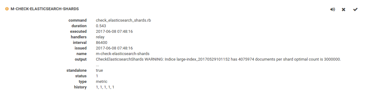
This is sensu check that runs 1 time per day and advises how indice settings should be changed.
Gains
After changing & reindexing all 46 indices reduced:
- slow query (>500ms) count from 7million to <200 thousand per week
- storage by 20%
- GC young generation collections close to average
- CPU usage to 15-20% from 30-50%
- data nodes from 16 to 15
- RAM usage by ~15%
References:
- https://www.elastic.co/guide/en/elasticsearch/guide/current/heap-sizing.html#compressed_oops
- https://www.elastic.co/guide/en/elasticsearch/reference/current/cat-shards.html
- https://www.elastic.co/guide/en/elasticsearch/reference/current/docs-reindex.html
- Elasticsearch shards matrix markdown generator