How Vinted Serves Personalised Search Autocomplete
At Vinted, more than 20% of all search sessions now start with a click on an autocomplete suggestion. A few years ago, that number was below 8%. Autocomplete not only saves typing effort - it helps people discover listings they didn’t know existed, and guides them toward successful searches.
Today, across 24 languages and 50+ country-language combinations, we have a pool of 125 million different queries ready to suggest to users. Our service, svc-suggestions, runs on Vespa and matches and ranks 4,700 queries per second at 31 ms P99.

Autocomplete systems work in two phases:
- Offline, we generate a pool of candidate queries - the things we might suggest - from product data, search logs, or both.
- Online, every time a user types a character, we match those candidates against the input (tolerating typos), rank the matches by what the user is most likely to click or buy, and return the top few. All of this has to happen in milliseconds - the bar is set by Google, Amazon, and every other product people use daily.
This post walks through each step - candidate generation from product metadata and search logs (and why 2% of candidates drive half the clicks), edge-ngram indexing for performance, fuzzy matching for typo tolerance, personalisation via a Learning-to-Rank model, and what 35+ A/B experiments taught us over two years.
Generating and scoring 125 million suggestions
The foundation of any autocomplete system is candidate generation - producing the pool of suggestions that will later be matched and ranked at query time.
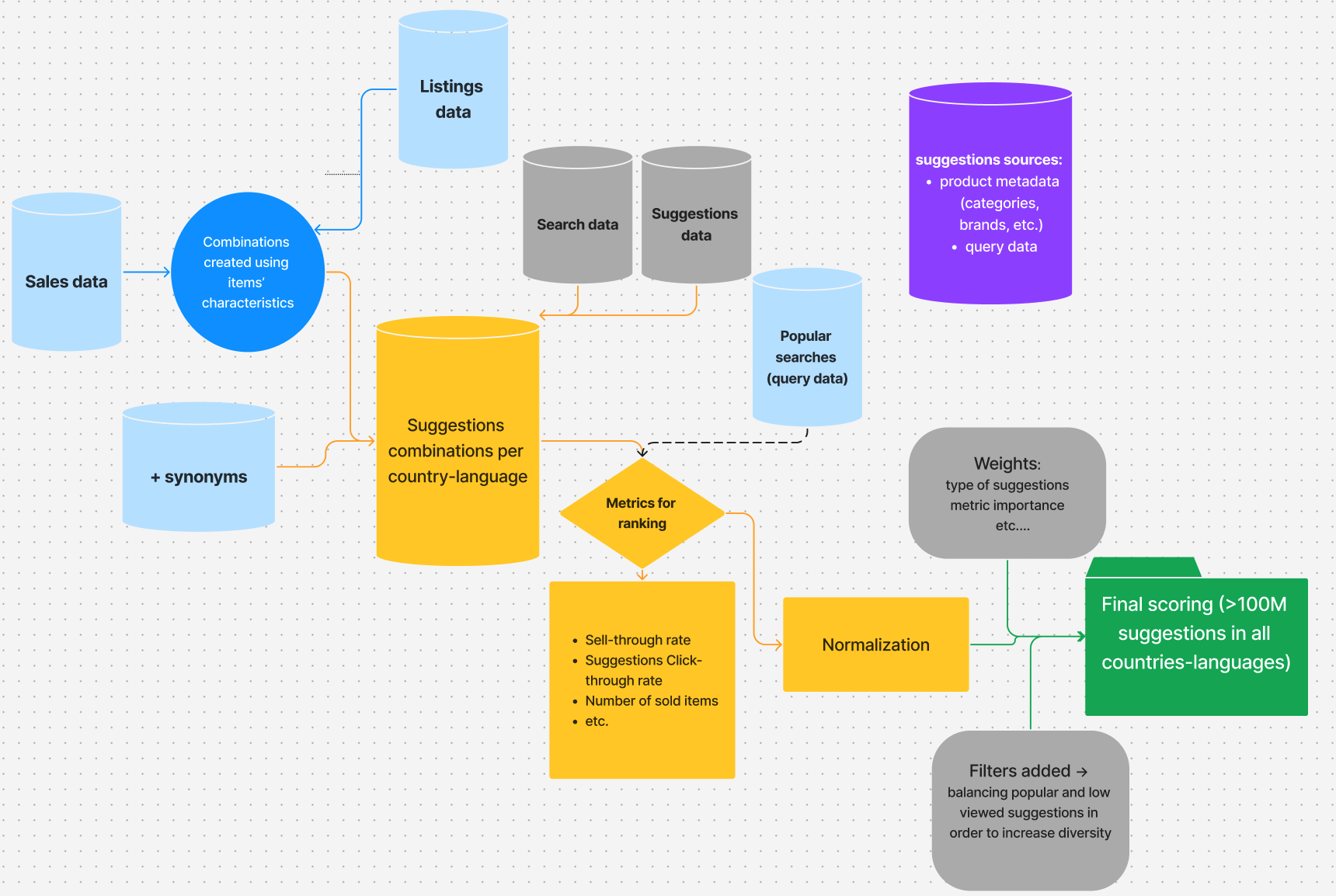
At Vinted, our Self-Learning Suggestions (SLS) pipeline draws candidates from two sources:
- Product metadata - item features such as category, colour, brand, and attributes are combined to generate all possible entity combinations (e.g., “Nike shoes”, “red dress Zara”).
- Search logs - popular user queries in each country-language market, capturing real demand signals and seasonal trends. These include queries that metadata alone could never produce, like book titles (“harry potter and the prisoner of azkaban”), holiday-related content (“world book day costume girls”), or fashion trends (“y2k baggy jeans”).
This dual approach ensures broad coverage: metadata-based suggestions surface inventory that users may not yet know to search for, while query-based suggestions reflect proven demand.
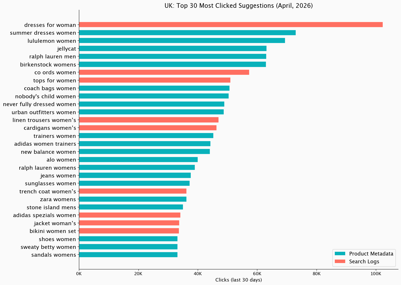
Below in the graph you can see UK’s most clicked suggestions in April 2026, by their source type:
In addition to this, we can see how product metadata and query logs shift with trends and seasons, using our members’ data. Let’s compare UK’s top clicked search suggestions during December 2025 and April 2026:
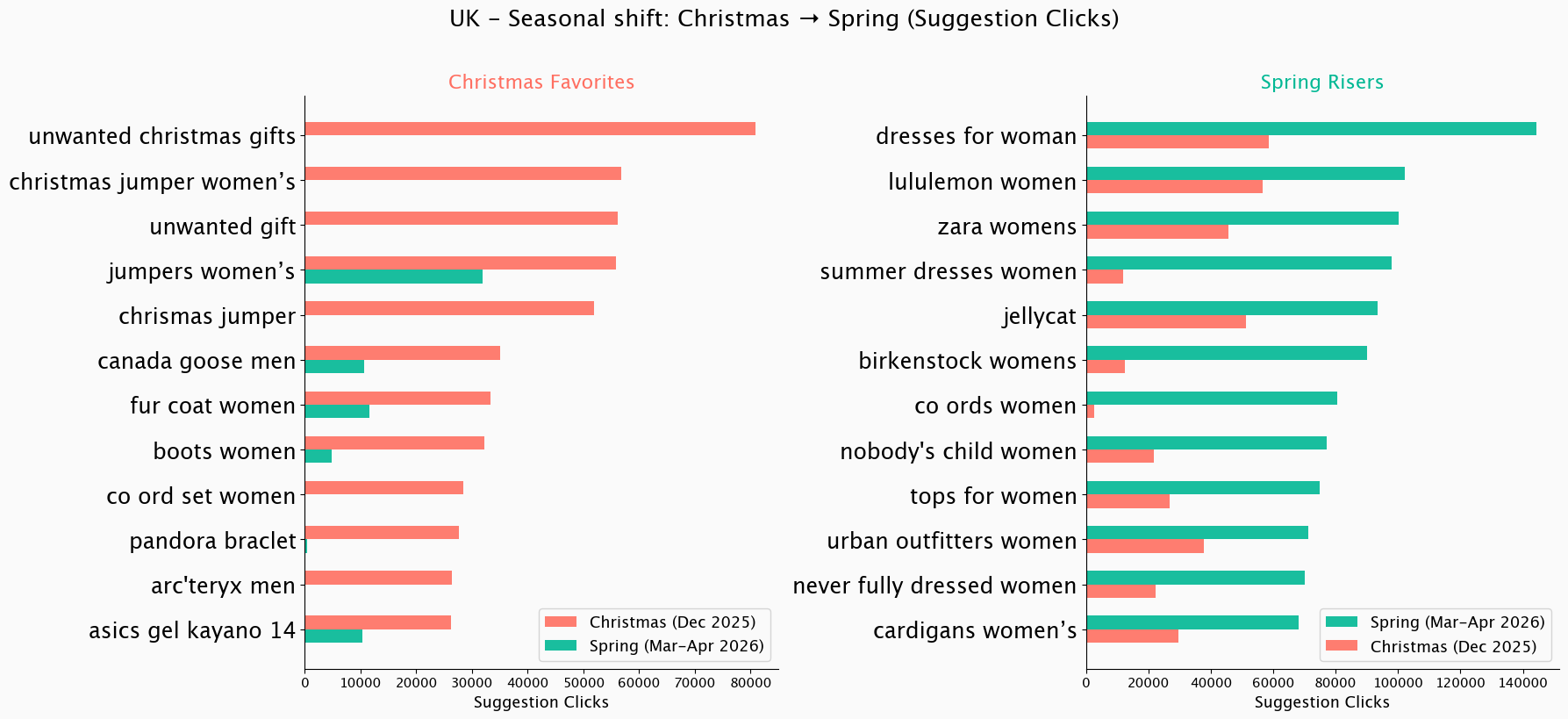
Seems like “unwanted christmas gifts” climbs into one of the most popular search suggestions in the UK during December. Nothing says “Happy Holidays!” quite like millions of users collectively speed-typing their way to rehome that lovely reindeer jumper or luxury mini spa set before New Year’s 😄.
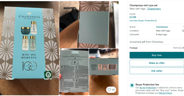
Multiple r/vinted threads show that reselling unwanted Christmas gifts is a recurring topic Vinted members discuss each year:

Candidate scoring
Once candidates are generated, they need to be scored. The SLS model computes a final ranking score for each suggestion using a multi-objective heuristic approach. It builds on the Most Popular Completion (MPC) framework [1], extended with our own metrics, normalisation, and weighting logic.
Several performance metrics are calculated per suggestion, including:
- Item STR (sell-through rate) - how often items matching this suggestion actually sell
- Number of sold items - absolute transaction volume behind the suggestion
- Suggestion usage - the share of search sessions where the user clicks on a suggestion rather than submitting their own typed query
- Suggestions CTR (click-through rate) - the ratio of suggestion clicks to number of suggestion lists shown
The model scores candidates using aggregated metrics (such as 7-day item STR and suggestions CTR) at the country-language level. This means the ranking reflects the preferences of the “average” Vinted user in a given market - typically a 25-35 year-old female living in a city, looking for affordable fashion. Great as a baseline. Blind to everyone else.
These raw metrics vary significantly in scale, so we normalise them in two steps: first, extreme values are capped using a sigma rule to prevent outliers from dominating; then, capped values are min-max normalised to a [0, 100] range. Normalisation is done per country, language, and first letter of the suggestion - so “Nike” competes with other “N” suggestions in the same market, not with globally popular suggestions starting with different letters.
Each normalised metric is then multiplied by a hand-tuned weight that controls its relative importance. Weights are only applied when a metric has sufficient data - for instance, the CTR weight kicks in only if the suggestion has been shown enough times; below that threshold, the metric contributes with reduced influence. Additional bonuses are added based on structural properties: the entity combination type (e.g., brand-only vs. brand+category), whether the suggestion is trending, and so on. The final score is a linear sum of all weighted metrics plus these structural adjustments, normalised once more to produce the total score that each suggestion carries into Vespa.
Finally, a diversity filter balances popular and low-viewed suggestions so that high-CTR items don’t dominate every market. Without it, newer or niche suggestions would never get the exposure needed to prove themselves.
The result is over 125 million scored suggestions across all 50+ country-language combinations, generated twice a week and ready to be indexed into Vespa, the search and ranking engine that also stores, matches, and ranks suggestions at serving time.
Indexing suggestions into Vespa
Suggestions are indexed through Vinted’s existing Search Indexing Pipeline - BigQuery exports to a Kafka topic, and Apache Flink streams updates into a dedicated Vespa cluster. The pipeline is fully streaming, so even though we only regenerate suggestions twice a week, we could switch to real-time updates without touching the infrastructure.
Why Vespa?
Vespa is the primary search engine at Vinted - we migrated from Elasticsearch in 2023 and have written about the decision on this blog. For autocomplete specifically, the deciding factor was ranking: Vespa provides native support for ranking expressions and ML inference in the serving path, which means we can run a LightGBM model per keystroke without leaving the search engine.
The tradeoff: Vespa is weaker than Elasticsearch/OpenSearch in lexical analysis - it lacks built-in edge-ngram tokenisers and the rich analyser chains we needed. We close that gap in the matching section below.
Matching user input in milliseconds
Once a user starts typing, we need to match their input against 125 million suggestions as fast as possible.
We first implemented autocomplete using Vespa’s native prefix query - the approach Vespa recommends in their official Search Suggestions sample app. It worked, but at Vinted scale our load tests revealed P99 latency around ~220 ms. Not good enough for autocomplete, where every millisecond of delay is felt and CPU is burnt.
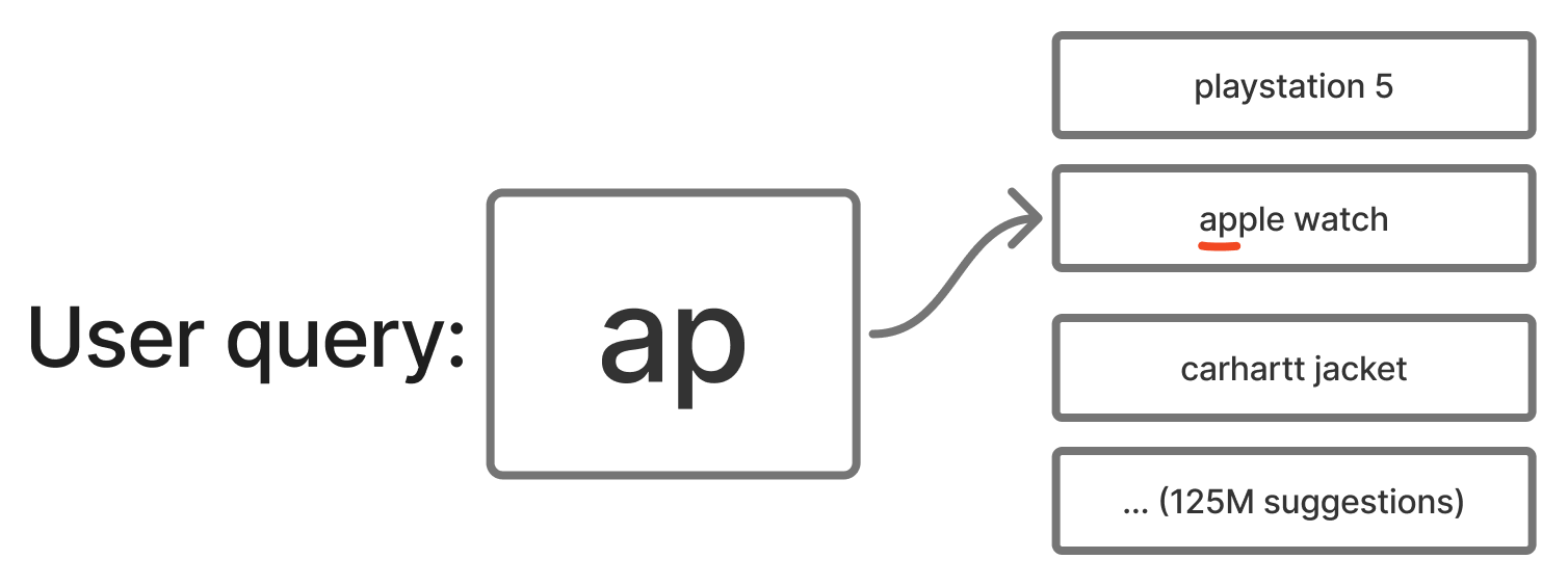
So we moved the matching cost from query time to indexing time. Borrowing the idea of an edge-ngram tokeniser from Elasticsearch, we split each suggestion into all its prefixes at index time:
"apple" → ["a", "ap", "app", "appl", "apple"]
At query time, matching becomes a simple contains lookup:
select * from suggestions where title_edge_ngrams contains "ap"
The suggestion text field is indexed in memory using Vespa’s attribute: fast-search. We brought the edge-ngram tokeniser into Vespa through Lucene Linguistics - our contribution to the Vespa project that allows Lucene analysers to run inside Vespa’s indexing pipeline.
The tradeoff is higher memory usage from storing more terms. For us it was worth it: P99 Vespa matching latency dropped from ~220 ms to ~25 ms, CPU usage decreased, and autocomplete felt faster for users.
Accent tolerance without losing intent
Vinted operates in many European countries, and a lot of languages use accented characters like š, ė, ą, ž, ł. In practice, users rarely type accents - instead of ž they simply type z - but we still want suggestions to match.
The naive approach: apply Lucene’s ASCIIFolding at both indexing and query time. ASCIIFolding is a token filter that maps accented Unicode characters to their closest ASCII equivalents (Ž → Z, ė → e, ł → l). This works for matching - but it throws away information. Typing an accent is a strong intent signal. If a user types Ž, they usually mean Žalgiris, not Zara.
To support this, we use a Multiplexer token filter, which stores two versions of every token:
- original accented token
- ASCII-folded token
So “žalgiris” is indexed as both “žalgiris” and “zalgiris” (each then further split into edge-ngrams: ["ž", "ža", ..., "žalgiris", "z", "za", ..., "zalgiris"]).
Typing Z matches the ASCII-folded token → finds both Zara and Žalgiris:
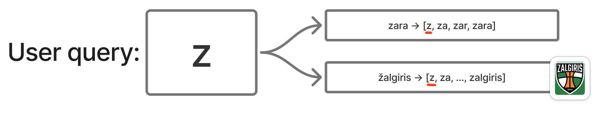
Typing Ž only matches the real accented token → finds Žalgiris only:

This gives us accent tolerance when users don’t type accents, while preserving intent when they do.
Handling typos with fuzzy matching
Handling misspellings is a must-have for autocomplete. Vespa provides fuzzy matching based on Levenshtein edit distance, allowing suggestions to match even when the user mistypes part of a word.
Two parameters control the tradeoff between fuzziness and performance:
maxEditDistance- how many total character edits are allowedprefixLength- how many prefix characters must match exactly (no edits allowed)
In our case:
prefixLength = 1- improves latency by reducing how many edit combinations Vespa needs to consider, and improves relevance by avoiding edits on the first character (changing the first letter often turns the query into a completely different word).maxEditDistance = 1 or 2depending on the fallback level. Edit distance 1 catches most common typos; we escalate to 2 only when the first pass returns too few results.
select * from suggestions
where title_edge_ngrams contains ({prefixLength: 1, maxEditDistance: 2} fuzzy("ap"))
When we started, Vespa didn’t support fuzzy prefix search - unlike Elasticsearch, where it’s built in. This was critical for us because users make typos before they finish a word, not only in finished ones. We opened a feature request, and the Vespa team shipped fuzzy on prefix:true shortly after - one of several fast turnarounds we’ve had with them on this project. By the time it landed, our edge-ngram design already covered the same ground: once prefixes are materialised as indexed tokens, Vespa never needs prefix:true mode for either exact or fuzzy queries. We stuck with edge-ngrams.
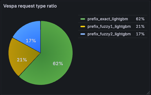
Cascading from precise to permissive queries
A single match pass isn’t always enough. For common queries, exact prefix returns plenty of results and the work ends there. For typos or unusual prefixes, we fall back through progressively more permissive matchers. Each additional tier is another client-to-Vespa round-trip on the hot path of every keystroke, so we order the tiers from most precise to most permissive and stop the moment we have 10 unique, deduplicated suggestions:
- exact prefix
- fuzzy (edit distance 1)
- fuzzy (edit distance 2)
Most popular queries produce 10 results in the first tier and never pay for the rest. Queries with a typo or an unusual prefix fall through to the next tier, stopping as soon as we have enough results.
This ordering also gives us ranking signal for free. Vespa doesn’t expose how many edits a fuzzy match used, so within one query we can’t tell an exact hit from a heavily corrected one. By splitting tiers we know the “strength” of a match from the phase that produced it, which lets us rank exact matches ahead of fuzzy ones when we merge results.
One deliberate design choice: we don’t relax aggressively. Returning nothing is sometimes better UX than something irrelevant. If we can’t suggest anything good, we let the user finish typing. If their query eventually succeeds, it enters the search logs and over time becomes a suggestion for everyone.
Most keystrokes never leave the first tier. Of all Vespa requests issued by svc-suggestions, ~62% are exact-prefix; the rest are split between the two fuzzy tiers.
Personalising ranking with Learning-to-Rank
The matching layer produces a ranked list of candidate suggestions using the SLS heuristic score. But heuristic ranking treats all users the same. To make suggestions personal, we added a second-phase re-ranking layer using a Learning-to-Rank (LTR) model that runs natively inside Vespa.
Model specifics
We chose a tree-based LTR approach using LightGBM with a LambdaRank objective, optimising directly for NDCG@1. LightGBM is fast at inference, memory-efficient, supports categorical features natively, and remains interpretable - all important properties for Vinted’s autocomplete system that must re-rank 20 suggestions per keystroke within milliseconds.
The model is trained on user-query-suggestion interaction data: for each query prefix, we observe which suggestions were shown and which ones users clicked. This produces labelled query-suggestion pairs that the model learns to rank.
Features
Our model uses 63 features organised into four groups:
| Feature group | Examples | Count |
|---|---|---|
| Query & Suggestion | Input length, suggestion length, entity type combinations | ~10 |
| Popularity | CTR, click count, total score, frequency ratios | ~15 |
| User Behaviour | Click history, purchase patterns, category preferences (e.g., fashion vs. electronics vs. high-value fashion), suggestion interaction patterns | ~25 |
| Contextual | Country, language, platform (iOS / Android / Web), month | ~13 |
Below you can see what the model actually learns (feature importance) and which features make the biggest impact:
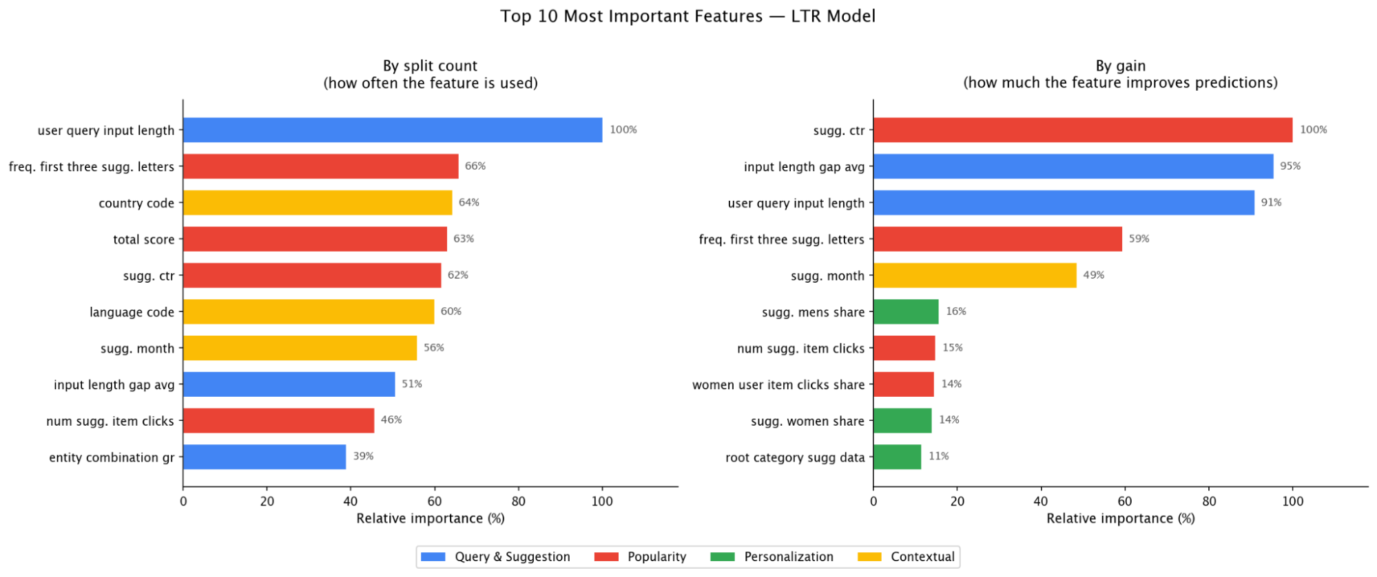
The single biggest signal is how much the user has typed - top feature by split count and top 3 by gain. Close behind are popularity signals: prefix-level click frequency, suggestions CTR, and the SLS heuristic score (4th by split - validating that the LTR model builds on the baseline rather than replacing it).
Equally important is the gap between current input length and when users typically click a given suggestion (top 2 by gain). The model isn’t just learning what to show - it’s learning when to show it.
User preference features - favourite categories, brand interests - carry less individual weight but work collectively. They appear in the gain top 10 but not in the split top 10: the model doesn’t check them often, but when it does, they meaningfully change the ranking - especially on short, ambiguous prefixes where generic popularity can’t distinguish intent.
Serving architecture
Vespa runs two-phase ranking on every keystroke:
- First-phase - SLS score. Each content node matches up to 1,000 candidates and orders them by the offline SLS score (described in Candidate scoring). This baseline is the same for every user in a given country-language market.
- Second-phase - LightGBM re-ranking. The top 20 per node are re-ranked by the LightGBM model inside Vespa, combining indexed suggestion-side features with user-side features fetched in real time from Vinted’s Feature Store (VFS).
Personalisation in practice
The model learns that different users want different suggestions for the same prefix. For example, when a user in the UK types “sh”:
- The baseline SLS ranking (same for all users) might show: “shoes”, “shirt”, “shein”, “shorts”…
- A user who predominantly clicks on men’s items sees: “shoes men”, “shirt”, “shacket”…
- A user who mostly browses women’s items sees: “shein”, “shoes women”, “shoulder bag”…
This is especially impactful for short prefixes (1-3 characters), where the candidate space is large and generic ranking struggles to surface what any individual user actually wants.
Making it work in production
Building the LTR model was not a straight path - over 20 model variations, 5 experiments, and results ranging from clear regressions on early iterations to meaningful lifts in the version that eventually scaled.
Not all problems were about the model. Early on, our LightGBM scores in Vespa didn’t match the offline ones - same inputs, different outputs. We suspected a bug in Vespa’s LightGBM lambdarank integration around categorical features, put together a minimal reproduction, and reported it. The Vespa team shipped fixes very quickly (vespa#34084, vespa#34094).
On the data side, the biggest win was deceptively simple: cleaning up noisy training labels. When users type short prefixes (1-4 characters), they’re still typing, not choosing. But our click attribution marked suggestions as “clicked” at these lengths even when the final click on a suggestion happened at later tokens. Stripping those noisy positives immediately improved ranking quality.
We also learned where not to re-rank. Initially, the LTR model scored all returned suggestions - including fuzzy and fallback matches. But fuzzy matches are already lower-confidence by nature, and re-ranking them alongside exact prefix matches muddied the results. Restricting LTR re-ranking to exact prefix matches only gave a clear boost to relevance metrics.
High-level architecture
Offline, BigQuery generates and scores the 125M suggestions, which Kafka and Flink stream into Vespa. Online, svc-suggestions fetches user features from the Feature Store, queries Vespa with progressive relaxation, and returns the top 10.
Vespa hardware
The Vespa clusters run in three European data centres - with US expansion coming - each with 6 content nodes organised as 2 groups of 3. Indexes are split per country, so a query touches only the country’s shard group. Each content node is an AMD EPYC 7713P (64 cores, 128 threads) with 512 GB of RAM.
Search CPU averages ~2% and peaks at ~4.5% during evening traffic (Western Europe evenings), even at 4,700 QPS. The write-CPU spikes are the twice-weekly index rebuilds, which push total CPU to ~7% on those days. The cluster has a lot of headroom: we could grow the user base, expand the suggestion pool, or run heavier ranking models without needing more metal.
Lessons from 35+ A/B tests
Over two years we ran 35+ A/B experiments (30+ on SLS, 5 on LTR), with a ~30% scale ratio. Our two primary engagement metrics were suggestion usage (share of search sessions that click a suggestion) and suggestions CTR.
A/B tests and interleaving
An A/B test at Vinted splits users into two groups - one sees the current autocomplete (“OFF”), one sees the change we want to evaluate (“ON”) - and we compare their behaviour: which group uses autocomplete more (suggestion clicks, session-level usage) and which group buys more on Vinted overall (transactions, GMV). A typical test needs a week or more of traffic before the numbers stabilise.
During periods of rapid iteration, we had more variants to test than A/B could handle in reasonable time. So we used team-draft interleaving: one list per user with suggestions drawn alternately from both variants, and we measured which variant’s suggestions users clicked more. We knew which variant was better in about a day instead of a week, which let us test ideas in batches.
Why evaluate engagement, not sales
Autocomplete sits at the very top of the search funnel. A user accepts a suggestion, gets a better query, finds a relevant item, and eventually may purchase. This path has many confounding variables (item and shipping price, seller responsiveness, recommended items, promoted items), and the signal diminishes at each step.
Industry literature confirms the pattern: even Amazon reports modest ~0.13% revenue lifts from QAC improvements [2], and most published work by eBay, Walmart, and Spotify [3][4][5] focuses on engagement metrics (MRR, acceptance rate, keystroke savings) rather than direct sales attribution. Sustained improvements in suggestion relevance and top-of-funnel engagement compound into better search sessions, discovery, and eventually conversions - but the causal chain is long.
A few notable tests
Out of 30+ SLS experiments, a few are worth calling out.
SLS: massively increasing autocomplete usage
Before SLS, Vinted’s autocomplete was a static list of brand and category names - no data-driven ranking and no real user queries in the pool. The first SLS version shipped in early 2023 in the UK; over two years and 30+ experiments, suggestion usage climbed from under 8% of search sessions to over 17%.
The first significant increase came in April 2023, when we scaled SLS in the UK, with a +0.9% lift in search GMV per active user and +0.7% in search transactions per active user. The plateau from May to September 2023 (~10%) covered multiple iterations to get SLS performing well across all countries and languages. The first big jump across the whole marketplace came when SLS was scaled to all countries (September 2023). The step-change in early 2024, from ~13% to 17%+, came from adding query-data suggestions - one of the biggest levers in the entire SLS journey.
SLS originally drew candidates only from product metadata - combinations of brand, category, colour, and attribute. This was a clear constraint: users search for things metadata can’t describe (e.g. “atomic habits”, “sony wh-1000xm5”, “charizard pokemon card”, “mob wife coat”), and without those queries in the pool, autocomplete felt out of touch with how people actually shop.
Adding user search queries to the candidate pool changed that. Query-based candidates make up only ~2% of the total pool but account for roughly half of all suggestion clicks - users gravitate toward suggestions that match how real people search.
The caveat: query data is only as good as the query volume behind it. It works best in markets with enough users to generate signal and enough inventory for those queries to return real results. In smaller markets, query data adds more noise than value.
Measured in short-term (<= 2 weeks) experiments, the cumulative impact of the full SLS system was:
| Metric | Result |
|---|---|
| Suggestions CTR | ~+49% |
| Suggestion usage | ~+42% |
| Search channel transactions | ~+0.8% (p < 0.05) |
Debounce: latency is a product feature
The app used to wait 350 ms after each keystroke before asking for suggestions - every new character would cancel the pending timer and restart it. We dropped that to 100 ms, below the threshold at which a system feels instant. In a four-variant test, 100 ms won cleanly: suggestions usage up ~12%, iOS session-level usage up ~15%, and manual typing (users giving up and typing the full query themselves) down ~4%.
Shorter debounce also means more keystrokes actually fire a request instead of being cancelled by the next character - meaningfully increasing QPS to Vespa.
Capitalisation: a deliberate tradeoff
A multi-variant test compared mixed-case suggestions (“Nike Shoes”) against all-lowercase (“nike shoes”). We believed that the casing should not affect user engagement metrics - but we were wrong - mixed-case had slightly better suggestions CTR and usage.
However, we had to make a deliberate tradeoff. Mixed-case broke visually when we started mixing metadata suggestions (which have predictable capitalisation) with query-data suggestions (which come in whatever case users type). Lowercase was less polished on individual suggestions but more consistent across the whole list, and could unblock future work. So we shipped lowercase anyway. Not every engagement win is worth scaling; sometimes the cleaner design is worth a point of CTR.
Scoped suggestions: richer UI, weaker conversion
We tested suggestions that carried a category scope - clicking one didn’t just run a query, it applied the category as a hard filter on the results page. Visually richer, two jobs at once (search and scope).
CTR was up ~2.4% and usage up ~2.7% against the no-scopes baseline. But the downstream numbers told a different story: users who clicked a scoped suggestion were ~1.3% less likely to buy in that session (statistically significant), and transactions per active user trended slightly negative. The scope was restricting the result set in ways that hurt conversion. We did not roll it out.
Looking at major e-commerce and search players today, almost all stick with a plain lowercase query list. Showing more per suggestion (categories, filters, thumbnails) is rare even at the largest scale.
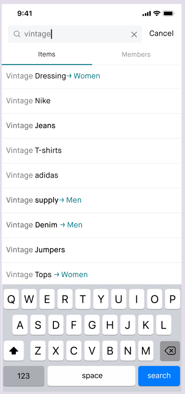
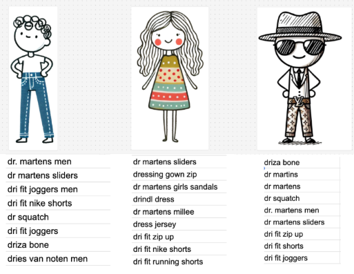
LTR: personalisation on top of SLS
With SLS producing strong baseline suggestions, the remaining problem was that every user saw the same ranking. A user who predominantly browses women’s clothing and one who shops for men’s luxury brands got the same list for the prefix “dr” (you guessed it - “dresses” often being the number one suggestion).
Five experiments over several months iterated on features, training data, and when to apply the re-ranking. The final model scaled to 100% of users.
Key results:
| Metric | Result |
|---|---|
| Suggestions CTR | ~+8% |
| Suggestion usage | ~+4% |
| CTR on longer queries | up to +16% |
| Avg. value of viewed suggestions (EUR) | ~+5% |
More interesting than the aggregates was multivertical visibility. The SLS baseline was implicitly biased toward clothing, the dominant category on Vinted. Personalisation surfaced non-clothing verticals - electronics, sports, high-value fashion, luxury, and home - for the users who actually wanted them. The sports vertical showed particularly clear downstream impact: transactions per active user up ~0.91% (p < 0.05), buyer GMV per active user up ~1.5%.
We also saw users deepening their relationship with autocomplete: clicks per user up ~3.8%, share of multi-day suggestion users up ~1.3%. Personalisation doesn’t just change a single session - it changes how much users lean on the feature over time. The effect on the suggestion-usage metric is obvious - across all countries we saw significant shifts, with countries newly onboarded to Vinted seeing the biggest increases.
Learnings along the way
Getting here meant building the SLS pipeline from scratch, migrating from Elasticsearch to Vespa, implementing edge-ngram indexing and progressive query relaxation, and layering on a LightGBM Learning-to-Rank model for personalisation. A few things during this journey stood out:
- Get the retrieval foundations right first. The Vespa migration and SLS generated suggestions doubled suggestion usage before we even added ML re-ranking. A solid baseline makes ML improvements additive, not a rescue operation.
- Don’t underestimate heuristics. The SLS heuristic baseline carried most of the usage lift before we added any ML - simple, well-tuned heuristic approaches go a long way.
- Real queries often beat the generated ones. Query data is a strong win when there are users and inventory to back it. Real search queries outperform machine-generated metadata combinations - but only when enough users are typing and enough items exist to make those queries useful.
- Personalisation pays off in the long tail. Its primary value lies in the long tail - the ambiguous queries where individual intent diverges from the average - which is not easily captured by aggregate business metrics. Patience and good experimentation infrastructure are essential.
- Engagement metrics are the right leading indicators. Suggestions CTR, usage, and keystroke savings are the most sensitive and reliable signals for autocomplete quality. Downstream business metrics follow, but take longer to materialise.
- Know when to show nothing. Our progressive relaxation and deliberate restraint on aggressive fuzzy fallback reflect that principle.
- Industry defaults exist for a reason. We tried richer visuals more than once - capitalisation, category scopes - and the results rarely beat plain lowercase suggestions that run a simple text search. Most major search players do the same. Novelty in autocomplete UI consistently lost to user familiarity with the basic pattern.
What’s next
With the retrieval, ranking and personalisation foundations in place for search autocomplete, here’s where we’re heading:
- Session-aware re-ranking - using the queries a user has typed earlier in the session as context for the LTR reranker. A user who just searched “nike air max” and then types “s” is likely after “shoes”, not “skirt”.
- Surfacing each user’s previous searches directly in autocomplete, drawn from both the current session and earlier ones. Google and eBay already do this - past searches render alongside popular suggestions, typically with a clock icon and an inline “remove” control.
- Neural suggestion generation - LLMs open up an exciting frontier for autocomplete: generating suggestions that no user has typed before and no metadata combination could produce. Be it long-tail queries, conversational phrasings, or trend-aware suggestions that adapt faster than any data logs based pipelines. The challenge, though, is latency - autocomplete fires on every keystroke under a 100 ms budget, so generative inference doesn’t yet fit the head traffic. But with smaller and faster models, smarter caching, and better serving infrastructure, this gap is closing fast. So we see LLM generation as a natural next layer on top of foundations we’ve built.
References
[1] Ziv Bar-Yossef, Naama Kraus. Context-sensitive query auto-completion. 2011.
[2] Sonali Singh, Sachin Farfade, Prakash Mandayam Comar. Evaluating Auto-complete Ranking for Diversity and Relevance. Amazon Science.
[3] Adithya Rajan, Weiqi Tong, Greg Sharp, et al. Semantic De-boosting in e-commerce Query Autocomplete. Walmart Global Tech.
[4] Enrico Palumbo, Gustavo Penha, Alva Liu, et al. AudioBoost: Increasing Audiobook Retrievability in Spotify Search with Synthetic Query Generation. Spotify.
[5] Hung Nguyen, Jayanth Yetukuri, Phuong Ha Nguyen, et al. Enhancing Related Searches Recommendation System by Leveraging LLM Approaches. eBay.